Quarks & Gluons

Roughly speaking, a gauge theory is a kind of physical theory which is invariant under local transformations based on some Lie group $G$ . The most important cases are gauge theories based on special unitary groups $SU(N)$ . Let me explain this previous sentence using the prototypical example of a gauge theory: Quantum Electrodynamics (QED) the theory that describes the interaction between electrons and photons.

QED

Free electrons and positrons are described by the Dirac Lagrangian (in God-given units) given by

${\cal L}_{e} = \bar{\psi}(i\gamma^\mu\partial_\mu - m)\psi$

where $\gamma_\mu$ are the Gamma matrices. The gauge group in this case is $U(1)$ and the Lagrangian above is obviously invariant under the global $U(1)$ transformations

$\psi\mapsto e^{-iQ\theta} \psi$ and $\bar{\psi}\mapsto \bar{\psi} e^{iQ\theta}$ (*)

where $\theta$ is a constant. Now, we would like to consider the local $U(1)$ transformations, and distinctive word “local” means that we should take the parameter $\theta$ as a position dependent object, that is $\theta=\theta(x)$ . In this case, the Lagrangian above is not invariant under the transformations (*), that is

${\cal L}_{e}\mapsto {\cal L}_{e} - i \bar{\psi}\gamma^\mu\psi \partial_\mu\theta(x)$

In order to recover the invariance of the Lagrangian under local transformations, we couple the Dirac field to the Yang-Mills Lagrangian for the abelian group $U(1)$ (although we generally use the terminology Yang-Mills just for non-abelian gauge groups). All in all, we have the Quantum Electrodynamics Lagrangian given by

${\cal L}_{qed} =-\frac{1}{4} F^{\mu\nu} F_{\mu\nu} + \bar{\psi}[i\gamma^\mu(\partial_\mu+iQe A_\mu) - m]\psi$

where $F_{\mu\nu}=\partial_\mu A_\nu - \partial_\nu A_\mu$ is the field strength. This theory is invariant under the local version of the transformations (*) provided the gauge field $A_\mu$ transforms as

$A_\mu \mapsto A_\mu + \frac{1}{e}\partial_\mu \theta(x)$

But we still need to give a physical interpretation to the vector field $A_\mu$ . But this is straightforward once we remember that $F_{\mu\nu}$ is just a covariant way of writing the electric and magnetic fields, it is the electromagnetic (or Maxwell) tensor.

Very enough, so using just symmetry arguments we managed to show that the Dirac Lagrangian should be coupled to a vector field $A_\mu$ that we have just seen is the photon. The coupling is given through the interaction term $i \bar{\psi}\gamma^\mu \psi A_\mu$ that in a quantized theory gives the following Feynman diagram vertex

qed-feynman-vertex-300x210

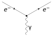
where the wavy line is the photon, the incoming straight line is the electron and the outgoing straight line is the positron.

Finally, one may notice that given the fact that the gauge group $U(1)$ has just one generator, namely, the functions $\theta(x)$ , implies that we need just one vector $A_\mu$ to couple to the Dirac spinor $\psi$ . In other words, the number of generators in the gauge group $U(1)$ is equal to the number of vectors $A_\mu$ . This explains why we have just one type of photon in the nature. Similar reasoning explain why we have 8 different types of gluons.

QCD

The next simplest gauge theory to consider is a theory based on the gauge group $SU(2)$ . I would like to write something on this theory since it is quite interesting and it appears in the context of the Higgs boson. Now I want to skip this case and study the third case. As you can imagine, the gauge group $SU(3)$ .

The theory describing the behavior of quarks and gluons, known as Quantum Chromodynamics (QED), is a gauge theory based on the gauge group $SU(3)$ coupled to six types Dirac spinors. These six types of Dirac spinors are, as you may imagine, the six flavors of quarks, namely, up, down, charm, strange, top and bottom.

Now, the Lagrangian for quarks is given by

${\cal L}_{quarks}= \sum_{f=1}^6\bar{\psi}^f (i\gamma^\mu\partial_\mu - m)\psi^f$

and the quarks $\psi_f$ transform in the fundamental representation (this is a phenomenological property of the fields) of the gauge group $SU(3)$ . In other words, each quark flavor can be mathematically represented as a 3 component column vector, that is

$\psi^f=\begin{pmatrix} \psi^f_1 \\ \psi^f_2 \\ \psi^f_3 \end{pmatrix}$ where $f=1,\cdots,6$

Equivalently, we write just the components $\psi_i^f$ where $i=1,2,3$ are indices in the fundamental representation of the gauge group. The gauge transformation is given by

$\psi_i^f=U_{ij}\psi_j$ where $U_{ij}\in SU(3)$

Around a small neighborhood of the point 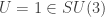$U=1 \in SU(3)$ we know that we can write this gauge group element as an exponential $U=e^{-i\Theta}$ and $\Theta$ is written in terms of the generators of the Lie group. In other words, around a small neighborhood of the Lie group $SU(3)$ , which is a manifold, it is enough to consider just the tangent space to this Lie group $SU(3)$ , its Lie algebra $su(3)$ .

Since $su(3)$ is, by definition of algebra, a vector space with basis $(T^a)_{a=1}^{dim(su(3))}$ , that satisfies the commutation relation $[T^a, T^b]=if^{abc}T^c$ and $f^{abc}$ are the structure constants of the Lie algebra. Now, we can write the parameter $\Theta$ in terms of this basis

$\Theta=\Theta^a T^a$ where $a=1,\cdots,$ dimension of $su(3)$

Ok, but what is the dimension of this space? This is easy to calculate. By definition, the group $SU(3)$ is

$SU(3)=\{M\in GL(3, \mathbb{C})|\det(M)=1\}$

with Lie algebra

$su(3)=\{A\in GL(3, \mathbb{C})|\mathtt{trace}(M)=0\}$

Therefore, these groups are spanned by $(3^2-1)=8$ generators. In other words, we have the 9 generators of the group $GL(3, \mathbb{C})$ of $3\times 3$ matrices, but we need to subtract the constraint coming from the unit determinant (or equivalently, the vanishing of the trace). All in all, we have that the Lie algebra $su(3)$ is an $8$ dimensional vector space.

We now can couple the gauge fields $A_\mu$ to the Lagrangian of quarks above. Repeating the analysis, we notice that the gauge field must be Lie-algebra valued and is written as

$A_\mu=A^a_\mu T^a$ where $a=1,\cdots, 8$

There are $8$ different types of gauge fields $A_\mu^a$ and these are, after quantization, the gluons. Since the field $A_\mu$ can be organized as a column vector of $8$ components, physicists usually say that it transforms in the adjoint representation of the gauge group, since this representation is realized as $8\times 8$ matrices. Moreover, an appropriate basis for the Lie algebra $su(3)$ is given by the Gell-Mann matrices.

The QCD Lagrangian is given by

${\cal L}_{QCD}=-\frac{1}{4}F^{a\mu\nu}F_{\mu\nu}^a + \sum_{f=1}^6\bar{\psi}^f [i\gamma^\mu(\partial_\mu-i g A^a_\mu T^a) - m]\psi^f$

where the field strength is $F^a_{\mu\nu}=\partial_\mu A^a_\nu- \partial_\nu A^a_\mu + g f^{abc}A_\mu^b A_\nu^c$ .

Finally, observe that the interaction between quarks and gluons is similar to the interaction between electrons and photons, in other words, we have the vertex $i \bar{\psi}^f\gamma^\mu \psi^f A^a_\mu$ , that in terms of Feynman diagrams is

qqbar-vertex-1-300x264

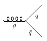
where the spring denotes the gluons and the $q$ and $\bar{q}$ represent one one the quarks and anti-quarks respectively.

However, the QCD has some new ingredients. Observe that contrary to the QED case, the gauge fields interact with themselves since we have terms of the form $\partial^\mu A^{a\nu}A_\mu^b A_\nu^c$ and $A^{a\mu}A^{a\nu}A_\mu^c A_\nu^d$ that give the Feynman diagrams

WorldOfGlue

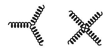
which give the possibility of the existence of bound states in the theory, known as Glueballs.

In conclusion, compared with QED, we see that QCD has many new features and for this reason it is much more interesting (and difficult). Furthermore, the quantization and the quantum treatment of gauge theories are challenging, since we need to be careful with the gauge fixing, Gribov copies, Faddev-Popov ghosts and other aspects of the theory. These are topics for other texts.

Some references

There are many good books on quantum field theory on this topic. In order to write this text I have used

That’s all folks!

M	T	W	T	F	S	S
						1
2	3	4	5	6	7	8
9	10	11	12	13	14	15
16	17	18	19	20	21	22
23	24	25	26	27	28	29
30	31

Quarks & Gluons

QED

QCD

One thought on “Quarks & Gluons”

Leave a comment Cancel reply

QED

QCD

Share this:

One thought on “Quarks & Gluons”

Leave a comment Cancel reply